Trouble with a formula in Numbers

[filmhandler]

So i have made this spreadsheet that tracks daily deposits, and when the file was in excel, I had a formula that made predictions of what the bank balance would be up to a week in the future. Now that I'm in Numbers, and I don't have a excel on my mac, that formula doesn't work. I need help to find a way to make the formula work, or a formula that will work.

the formula is this;

=if(B3=$A$1, $A$2 + C3, D9 + C3)

A1 has the formula for date of =NOW() and is formatted for Days of the week, Sunday - Saturday.
B3 through B9 are the days of the week
A2 is the current daily Balance
C3 through C9 is the Average daily deposit
D3 through D9 are the formula above copied and pasted so that the appropriate cells are referenced.

Can anyone help.

 

[MacInWin]

One problem I see in the formula is the D9+C3 expression. If that is in the D3 block, then D9 points to the last entry, but in the D4 block it points to D10, which is out of the data range. Or is the formula as you posted it what is in D9? In that case, the argument is circular. You have D9 being added to C3, then put in D9 which is added to C3, which is put in D9.... You can't do that.

 

[filmhandler]

the Expression of D9 + C3 will change on the following cell to D3 + C4. Either way it looks, the formula works in excel and google spreadsheet, and it doesn't in numbers.

basically it goes this;

=if (b3 {day of week} = $A$1 {Current Day of Week}, $A$2 {Current Bank Balance} + C3 {Day of week's Average Deposit}, D9 (Previous Day's Expected Deposit} + C3 {Day of week's Average Deposit})

As long as the day equals the current day, that day will have the lowest estimated balance, and the previous day will have the highest estimated deposit.

 

[MacInWin]

Well, check your formula on your spreadsheet. I entered that exact formula into Pages and it worked perfectly. Instead of typing it in, I used the point/click method to select the cells for the formula, the only difference I saw was that the "$" in front of the "A" was not there, so it ended up as "A$1" instead. But since you aren't copying it across columns, just down rows, that's essentially the same.

 

[filmhandler]

My problem is once I get the formula into all the cells. As soon as I have it in all the cells, i get a circular error. The error reads, "The Formula can't reference it's own cell, or depend on another formula that references this cell." It's like the IF condition is always coming back false, and it's only doing the final step.

 

[MacInWin]

Yep, you cannot have a circular reference. So when you link all of them in a chain, you get a circular reference. You need to somehow break the chain, maybe by putting the current balance into a cell NOT in the D3-D9 range.

 

[filmhandler]

The current Balance is in a cell all on it's own, it's not in the chain. That is the beginning of the formula, but for reason it doesn't calculate the true statement. I just can't find out why this formula works in Excel and Google Spreadsheet, but not numbers. It's a 7 day predictive balance formula. It takes the current balance and adds the average for the each day of the week to it.

So, if today is Monday, the Balance will have a projected balance at the end of the day of Current Balance, which comes from a complete separate set of data, plus the Average Deposit for Monday (C3). Now if today is Wednesday, you can look to see what your Projected Balance will be on Monday (D3). Because today is Wednesday, it should take Thursday, Friday, Saturday, Sunday, Monday and Tuesday and adds their average deposit individually to Wednesday's projected end of day balance in order, STARTING from the Current Balance (A$2). When the day changes from Wednesday to Thursday, the rotation to change again and take Friday, Saturday, Sunday, Monday, Tuesday and Wednesday, Starting from Current Balance.

Here's another Example.

Monday
Current Balance: $251,685

Sunday Avg: $4,968 False: Saturday Projected + Average $4,968
Monday Avg: $6,246 True: Current Balance + Average $6,246
Tuesday Avg: $6,843 False: Monday Projected + Average $6,843
Wednesday Avg: $6,538 False: Tuesday Projected + Average $6,538
Thursday Avg: $6,647 False: Wednesday Projected + Average $6,647
Friday Avg: $8,346 False: Thursday Projected + Average $8,346
Saturday Avg: $12,346 False: Friday Projected + Average $12,346

Saturday
Current Balance: $294,467

Sunday Avg: $4,968 False: Saturday Projected + Average $4,968
Monday Avg: $6,246 False: Sunday Projected + Average $6,246
Tuesday Avg: $6,843 False: Monday Projected + Average $6,843
Wednesday Avg: $6,538 False: Tuesday Projected + Average $6,538
Thursday Avg: $6,647 False: Wednesday Projected + Average $6,647
Friday Avg: $8,346 False: Thursday Projected + Average $8,346
Saturday Avg: $12,346 True: Current Balance + Average $12,346

I'm just confused as to how it doesn't work in numbers but it works in google sheets and excel.

 

[MacInWin]

You gave this formula

=if(B3=$A$1, $A$2 + C3, D9 + C3)

as the problem child. What cell is that particular version of the formula entered? If D9, then you have a circular reference.

And you don't have to keep explaining the problem, I understand what you want to do. But if that version of the formula is in D9, it's circular.

 

[filmhandler]

Okay, then can you help me find a setup that will achieve what I'm looking for?

 

[MacInWin]

The problem is that what's in D3 depends on D9, and what's in D9 depends on D8, D8 depends on D7, D7 depends on D6, D6 depends on D5, D5 depends on D4, D4 depends on D3, but D3 depends on D9, so it goes circular. In testing in Excel, I think the loop is broken by the existence of one TRUE statement, which no longer refers to the previous cell, but if that TRUE statement is missing, the same error appears in Excel. Try it yourself. Blank out A1 in excel and you get an immediate error message saying it's circular. I guess maybe Numbers tests BEFORE the true/false assessment and sees the circularity that way, while Excel tests the truth of the statement before assessing circularity. Frankly, Excel's approach is less correct than Numbers, but your spreadsheet takes advantage of that weakness in Excel.

I have thought about it some, but cannot think of a simple way to avoid the circularity. Everything I try keeps coming back to the circular argument. The only way out I can see is to build a table with days across the top and days down the side. In each cell is the amount of money that would be needed to be added to today's balance to forecast to the date in the week the next time it happens. If the average deposits for each day are subject to change, build that table with references to the averages, don't hard code the values. Then a combination of vlookup or hlookup should let you fetch the amount from the table based on the current day of the week and the date being forecasted. As I said, not simple.

Good luck with it. I'm not a Numbers wizard, maybe someone more experienced in it than I can figure out how to get around the circular reference. Too bad Numbers didn't have the loophole (bug?) Excel does.

 

[MacInWin]

OK, I've got a solution. It's a bit of a kluge but it works. Duplicate column D into Column E, then in D, delete D9 to be empty. Now in E, delete E3 to be empty. Now edit the formulae in Column E to fix them to reference Column B and C properly. Now create a column F and in F3 put this formula:

IF(D3>E3,D3,E3)

and copy that down from F3 to F9.

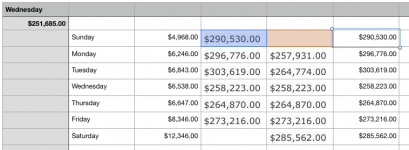
Now you can hide columns D and E and what's left, that is, F, will show the numbers you want to show. Or you can leave D and E showing and just use F for the forecast numbers. What this approach does is break the circularity in D and E by leaving one day out, and then letting F pick the larger of the two columns as the correct forecast number. Each day is correct in both columns after the current day of the week, but then E is incorrect BEFORE today's day of the week because E3 is zero, so the formula picks D instead. The missing days are 0, so the other column is selected. Here is how it ends up looking (I didn't hide D and E so you can see how it works):


I did test this by typing in the day of the week in A1 and each time it correctly selected the right value for F.

Hope that helps.

 

[filmhandler]

Amazing Jake,

I was looking around many places for a solution, and just happened to find that you replied again. surprisingly I didn't get the notification you had. This helps me tremendously.

I might have found why this works in excel and google spreadsheet, as I had a chance to examine the file in excel and I found that the cell A1 had a formula as this =TEXT(NOW(),"DDDD"). I'm not sure if that's what caused the circular error to disappear, or if it was something else, because I don't see any difference in the sell layout or formulas.

Amazingly it works now and I can't thank you enough!!!.